 Here is a fun situation everyone has thought of before… There are two populations on an island, a population of frisky beach bums who eat coconuts all day, and a population of man eating koala bears. The question is, what is going to happen over time? Will the people flourish and eat coconuts forever? Will the ravenous koalas devour all the people? Or can they somehow live together in a coconut/man eating harmony?
There have been many approaches to look at this problem, some very robust and thorough, and other simpler ones that just express the fundamental relationships. I’m going to take the latter route and make some slightly unrealistic assumptions to simplify the model.
- There is a magic golden palm tree which never runs out of coconuts. In other words, this island has an unlimited amount of coconuts, so the beach bums have an unlimited food supply.
- Second assupmtion, the man eating koalas only eat the beach bums. There is no other source of food for them on the island.
- There is no threat to the lives of the beach bums other than the carnivorous koalas.
So let’s define a few variables and see whats going on here.
 number of beach bums
 number of koalas
Since we’re speaking of populations it would be good to examine how the growth and decay vary for both the beach bums and the koalas. Let’s take a look at the beach bum population. The only way their population can grow is through procreation, which is dependent on the size of their current population, and the only way their population can decline, is from the frequency of crazy koala attacks, which is dependent on the current size of the koala population. In other words, or in math lingo to be precise…

Here alpha is the growth rate for the beach bum population. What does it depend on?
We need to consider how the population could grow, and how it could decay. For it to grow they would simply need to be the frisky beach bums they are and be left alone with their coconuts. So under assumptions (1) and (3) if there were no koala population, the beach bum population would grow exponentially without bound according to some friskiness constant, which we’ll call  .
.
However, if there is a koala population then some of these beach bums will be getting gobbled up. The number of beach bums to disappear must rely on the number of koalas that are hungry. So we can say the rate with which the beach bums die is proportional to the number of koalas times some hunting efficiency constant which we’ll call  .
.
So after some consideration and looking at our assumptions, alpha appears to be a function of the koala population which looks like this.

This then means that our differential equation expressing the life of the beach bum population is a function of both the current koala and beach bum populations, which now looks like this.

Using very similar reasoning, we know the koala population’s growth or decay should depend on it’s current population as well.

The question is, what does beta depend on? How does the koala population grow? Well they need to eat, so the more they eat the more energy they have, the more energy they have, the less time they need to worry about food, and the more time they can dedicate to their wives and to makin’ babies. In other words, the koala population will grow depending on their current population times some hunting efficiency constant which we’ll now call  .
.
According to assumption (2) how they die should be pretty clear. There is no other food source for the koalas on the island besides beach bums, so if there are no beach bums, then the koalas can’t eat and they begin to die. In other words, without a food supply the koala population will die at a rate proportional to it’s size. Again we’ll call this constant  .
.
We now know what beta looks like.

Here we know that the ODE representing the life of the koala population is also a function of both the current beach bum and koala populations.

After consideration and analysis, we’ve designed our math model. These two equations together happen to comprise the classic Lotka-Volterra Predator-Prey model.


Alfred Lotka and Vito Volterra
Let’s summarize these equations one last time.
 and
and  control the growth rates of their respective populations. They encompass the difference between the birth and death rates. These constants should be chosen while considering their natural growth, like their natural reproductive cycles, and some natural ways for the population to decline, say old age, or accidents for example.
 and
and  both represent hunting efficiency. This is because the more efficient the blood lusting koalas are at hunting, the more beach bums they will eat. The more beach bums they eat, the quicker the beach bum population decays and the faster the koala population grows.
Now that we’ve designed our model, the hard part is over and we can begin to examine it and learn about how the beach bums and the koalas play together. There are plenty of questions to ask. The first of which I find most interesting will be, can the beach bums and koalas coexist? This means we’re looking for equilibria, or points where neither population grows nor decays. We certainly have the obvious solution (0,0). If both populations are extinct then neither population will grow nor decay, this however isn’t a very interesting solution.
So what would it mean for neither population to grow nor decay? That would mean their derivatives should equal 0. This is where we consult our equations.


For clarity I’d like to point something out. Fixed points, critical points, equilibrium points, and stability points, all refer to the same thing. So for the rest of this discussion, we’ll show off our vocabulary and throw these different terms around quite frequently. Plus it’s good to be verse with math jargon so you don’t get confused when discussing things with colleagues!
We can see that we need both  and
and  to equal 0. For this to be true, either
  and
and  could both be zero or
  and
and  could both be zero.
If both  and
and  were zero we’d get the trivial solution again (0,0) which despite it’s boring nature is of some importance and will be considered later. Let’s examine the case then when both
  and
and  are zero!


So there are two points, particular populations of beach bums and koalas, where the derivatives are zero at (0,0) and  . The next natural question is to ask what is going on at those points? Apparently the bums and koalas can live together in some sort of harmony when there are
  beach bums, and
  koalas, however once the populations reach this point, will they remain stable over time? How exactly is the solution behaving around that particular point?
To analyze the behavior of non-linear systems near their critical points a common approach is to first linearize it, then examine the eigen values from the Jacobian matrix at each stability point. Particular sign combinations of the eigen values will tell you the nature of those stability points.
The first thing to do is linearize the equations. Remember a linearization is just a linear approximation of a non linear equation. Let’s flash back to multivariable calculus and drudge up these old equations.


Now these are only true when  and
and  are “sufficiently close” to
  and
and  . We’ll skip the details of what sufficiently close means here. Basically it needs to be close enough so that our linearization can accurately approximate the equilibrium point, so when
  , we also need
  . This leads to the following system.

This here is a good looking linear system just as we wanted. We can rewrite the system like so.


The matrix A in our linearized system above is the Jacobian matrix. The questions we have are concerning our equilibria and to analyze the topology around them all we need is to evaluate the Jacobian at the fixed points and find the eigen values. Below is the Jacobian.

Where all of the partials are equated as follows…


Substituting in the partials, the Jacobian turns out to be

Now we can study the behavior of the system near both the fixed points (0,0) and  . First let’s evaluate the Jacobian at the origin and find it’s eigen values, then from the eigen values we’ll know what the system is doing near that point.

The determinant is calculated as follows.


So we see that both  and
and  are equal to
  and
and  respectively. This is all we need to examine the behavior of the solution near the equilibrium point.

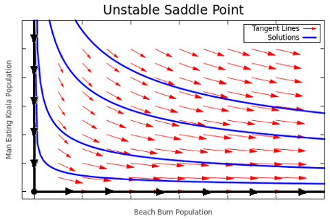
Topology for unstable saddle point
Our eigen values are of mixed sign so the critical point (0,0) is a saddle point. The topology for the critical point at (0,0) can be seen int the graph to the left. This is a graph of

vs.

which was generated with
gnuplot.
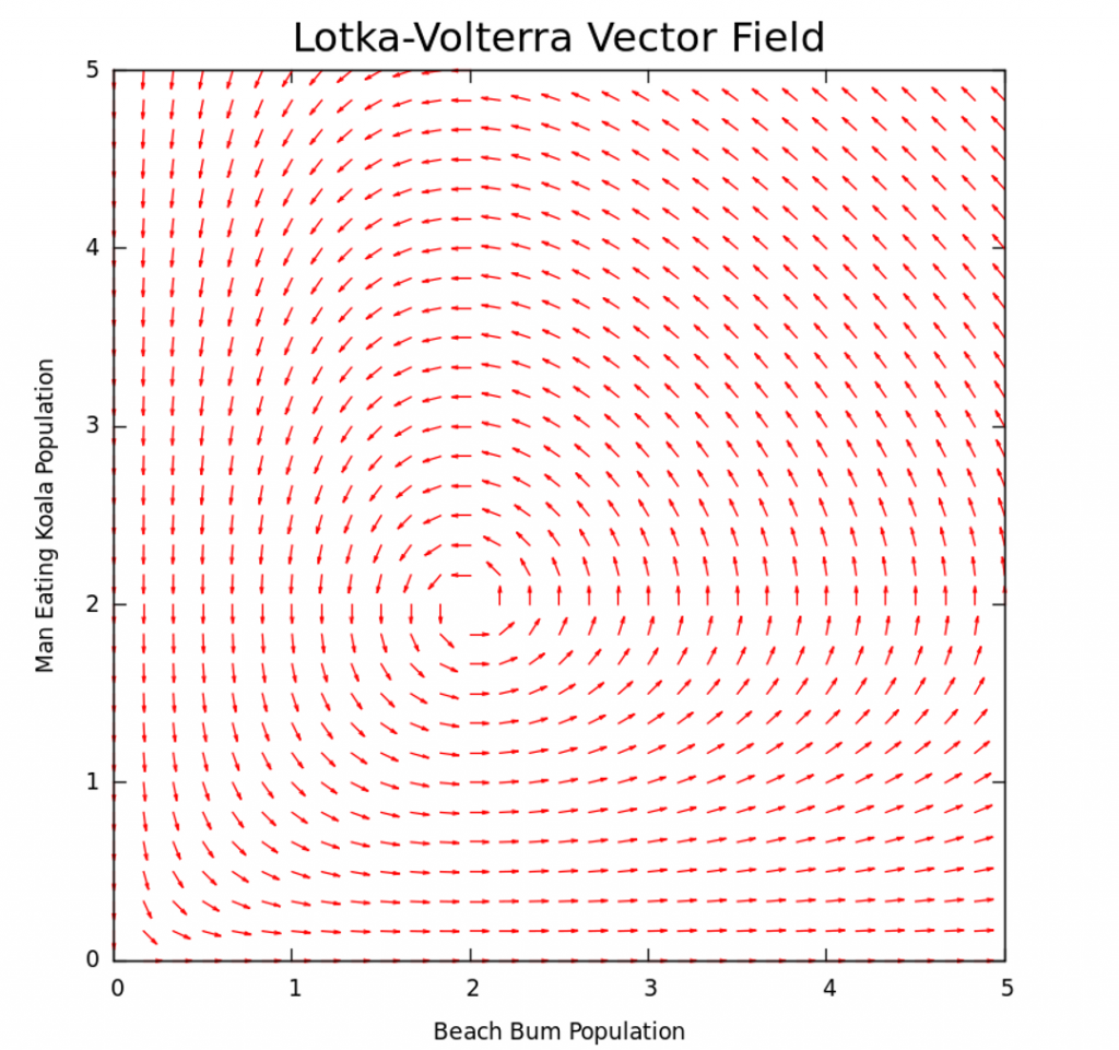
This is called a phase plane diagram. It shows us how certain solutions behave over time. The blue lines are called the trajectories, and they form the solution set. The red arrows form the vector field which shows the general flow of solutions over time. This is because every vector is tangent to a solution at the point of their tail. The straight line solutions in black are the eigen vectors corresponding to the eigen values we found earlier. We find two solutions along these lines. The one heading towards the origin as t increases is whats called the stable manifold while the other which goes away from the origin is the unstable manifold. This fixed point is unstable.
We said before that even though the physical interpretation of this stability point isn’t of much interest, the extinction of both populations, studying the behavior of other solutions around it is. Notice that any solution NOT on one of the straight lines never actually reaches the (0,0) point. This means that given two starting populations where neither are 0, then neither species will become extinct.
The solutions along the straight lines tell us something as well. The solution heading toward the origin tells us a story about what happens when a non-zero population of koalas exist on the island without beach bums. They quickly starve to death. However the straight line heading away from the origin tells the opposite. This is what happens when a non-zero population of beach bums exist on the island without koalas. They eat and have lots of sex, and as you’d think the population grows without bound.
Let’s examine the Jacobian at our other equilibrium point  . Again, the Jacobian looks like this.

So evaluating it at  yields…

To find the eigen values for this matrix we must find the zero’s of the characteristic polynomial, and the characteristic polynomial is given by finding the determinant of this matrix.

The determinant of this matrix is calculated as follows.


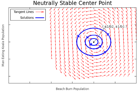
Both of the real components of the eigen values are zero, this gives us what’s called a center. All the solutions near the fixed point revolve around it periodically.

Topology of solutions near the point ( a2/b2, a1/b1 )
The graph to the right shows the behavior of solutions within a neighbor hood of the critical point  . Again, the red arrows show the general behavior of solutions within this area, while the blue lines are actual solutions. The tails of red vectors are all tangent to solutions.
We can interpret this as telling us the populations will oscillate with various amplitudes around the stability point and eventually come to a semi-stable oscillation. Physically this means that the koalas will eat a bunch of bums, then the koala population will grow larger than the bums, and the koalas will start to die off. Then after the koalas die off, the beach bums will begin to populate again, then once the population is large enough, the koalas will have an abundance of food and begin eating them at a frequent rate, where once again they will eat too many and the cycle will continue.
A good question from here is how do the fluctuations in population for both the beach bums and koalas relate to one another? Well take a look at the center point again. The  axis represents the beach bums population, it reaches it’s maximum when the koala population is at equilibrium. The koala population,
  , reaches it’s max when the beach bum population is at equilibrium. That’s 90 degrees from the horizontal axis to the vertical axis, so these solutions are 90 degrees out of phase!
It should make sense now to view the solutions of each equation as sinusoidal waves. The population of the predators grows as the prey begin to decline, then the prey’s population begins to grow back while the predators are still dying off from over hunting. Once the waves are superimposed over each other they should be about 90 degrees out of phase.
Getting a Better Understanding of the Solutions
If we were to combine both of the stability points onto one phase plane we’d get a really good idea of what is actually going on. If you’re curious about it, I wrote a program that does exactly that! If you want to see it in action, I made a video showing it off in the next post.
Predator Prey Models in Real Life
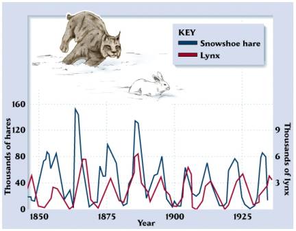
Now what’s truly exciting is this, we made a lot of assumptions when deriving this model, and even still the information extrapolated from this model can be found in actual physical models. The most popular example is the population of the snowshoe hare and the lynx.

Relationship between Snowshoe Hare and Lynx populations
As you can see observing how their populations have varied over 75 years has produced results very similar to those predicted by this model. The peaks between each population seem to be about 90 or so degrees out of phase from on another.
There exist much more robust models that can do an even better job of predicting the cyclical growths of predator-prey populations like these. After this introduction to how the process of modeling populations is approached, I hope you take the initiative to explore some of these more sophisticated models, and perhaps take a stab at designing a few of your own!
References
Dr. Kopriva’s Math Modeling Course
Paul’s Online Math Notes
Differential Equations and Chaotic Systems in Science
S.O.S Math


